

A Visual Guide to LLMs (Part 2)
Inside the Transformer Architecture.

In this two part series, we will go through the core components of Large Language Model (LLM) architecture step by step, making it easy to understand, even if you are new to AI.
Series Roadmap
Part 1: This part will show how written language is split into tokens and then turned into input embedding vectors that a model can work with. It explains tokenization, token embeddings, and positional embeddings.
Part 2: This part will show how those input embedding vectors move through the transformer block to produce output. It covers self attention, causal self attention and masked multi-head attention mechanisms, feedforward neural networks, how the next token is chosen, and how training slowly improves the model over time.
In A Visual Guide to LLMs (Part 1), we learned how Large Language Models (LLMs) take human language and turn it into something machines can understand. We took the sentence, “Every moment is a beginning,” sliced it into tokens, assigned them numerical IDs, and converted them into dense vector representations called token embeddings. We also added positional embeddings so the model knows the exact order of the words.
In Part 2, we will explore: the Transformer Block and the Output layer.
Now, I will explain each component of the Transformer block one by one.
One of the most important components is Masked Multi-Head Attention. However, before we get to that, we will first look at the Self Attention and Causal Self Attention mechanisms. Understanding these concepts will make it much easier to fully grasp how Masked Multi-Head Attention works. We will also cover Feedforward Neural Networks, Residual Connections, and Layer Normalization to understand how all the components of a Transformer block work together.
1. Self Attention Mechanism
Language is highly contextual. If you read the word “beginning,” its exact meaning depends heavily on the words that came before it. The self attention mechanism allows the model to understand how words relate to each other. Instead of reading each word in isolation, every token looks at the other tokens and decides which ones matter most.
In Part 1, we already created Input Embeddings after summing token and position embeddings.
Example: Every moment is a beginning
Token IDs: {”Every”: 15745, “moment”: 4205, “is”: 382, “a”: 261, “beginning”: 10526}
Final Input Embeddings (Sum of Token Embeddings + Positional Embeddings):
“15745” (position 1): [-0.5880, 0.3486, 0.6603] + [-0.9178, 0.9045, -2.0975]
“4205” (position 2): [-0.2196, -0.3792, 0.7671] + [1.1558, -1.2157, 0.1295]
“382” (position 3): [-1.1925, 0.6984, -1.4097] + [ 1.0937, 0.2066, 3.1815]
“261” (position 4): [ 0.1794, 1.8951, 1.3689] + [ 0.0967, 1.4086, 0.1915]
“10526” (position 5): [-1.6033, -1.3250, 0.1784] + [ -0.1562, 0.2446, 4.0124]
After performing element wise addition:
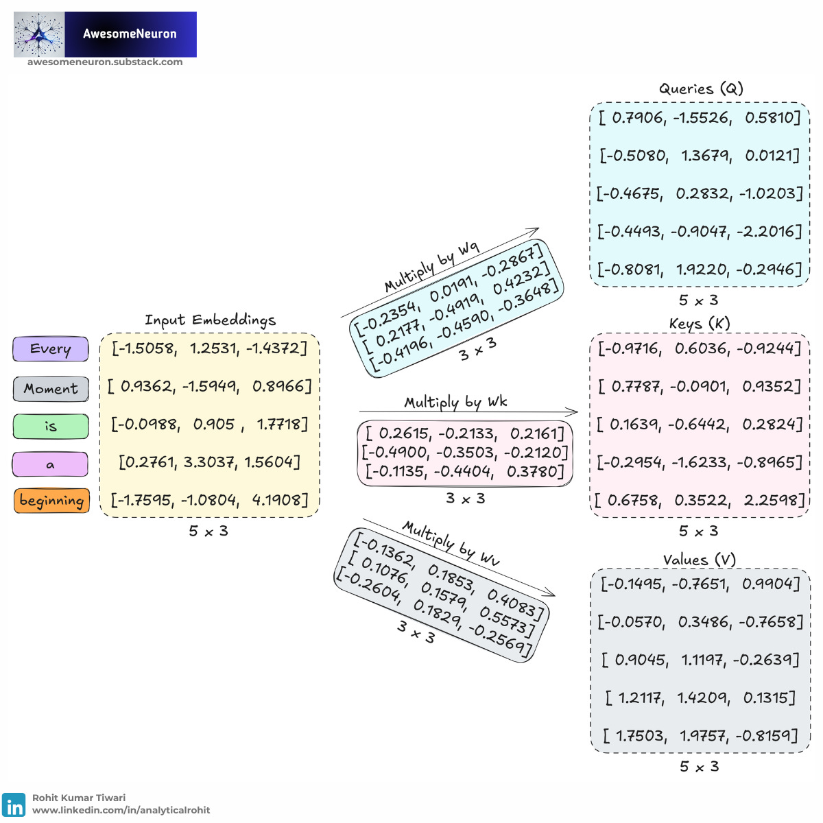
“15745” (position 1): [-1.5058, 1.2531, -1.4372]
“4205” (position 2): [ 0.9362, -1.5949, 0.8966]
“382” (position 3): [-0.0988, 0.905 , 1.7718]
“261” (position 4): [0.2761, 3.3037, 1.5604]
“10526” (position 5): [-1.7595, -1.0804, 4.1908]
To understand the word “beginning” in our sentence, the model pays attention to words like “moment” and “Every”. This gives context and helps the model capture the idea that each moment can represent a fresh start.
Step 1: To achieve this mathematically, the model uses three vectors derived from the input embeddings: Queries (Q), Keys (K), and Values (V).
Step 2: We compute the dot product between all Queries and Keys to measure how well they match.
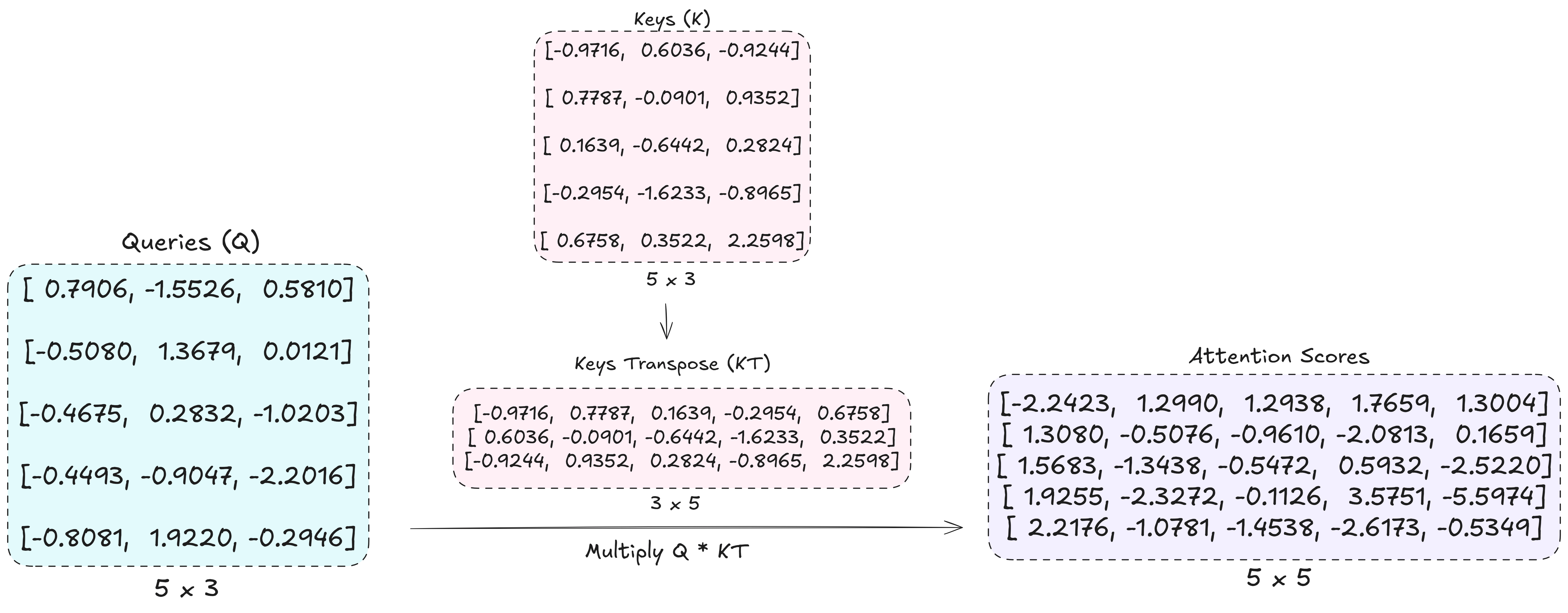
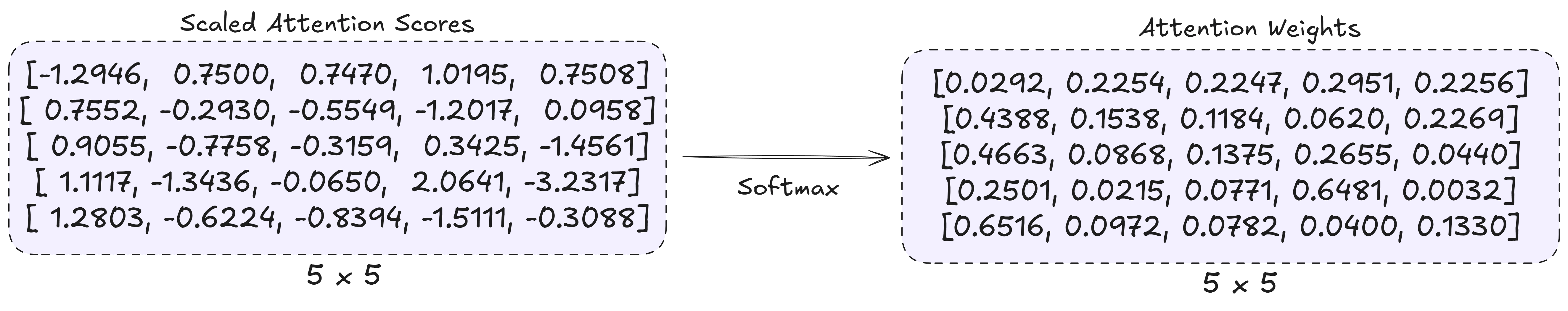
Step 3: The result is scaled by the square root of the key dimension dk to keep values stable during training.
Step 4: Apply softmax to obtain attention weights.
Step 5: Calculate context vectors.
Complete Self Attention:
After attention each token now contains information gathered from other tokens in the sequence. This is the core idea behind transformers.
Causal Masking: Hiding the Future Tokens
In standard self-attention, each token can attend to all other tokens. But in language models generating text word-by-word, future tokens should not be visible during prediction.
Causal self attention mechanism uses a mask to prevent tokens from attending to future tokens. The allowed attention pattern forms a lower triangular matrix, ensuring that each token can attend only to itself and earlier tokens in the sequence.
1 means attention is allowed.
0 means attention is blocked.
This is implemented by masking the blocked positions and replacing their attention scores with negative infinity before applying the softmax function. After softmax, these positions receive a probability of 0, preventing the model from attending to future tokens.
This ensures:
Token 1 sees only itself.
Token 2 sees tokens 1 and 2.
Token 3 sees tokens 1, 2, and 3.
Now each token can only attend to itself and previous tokens.
Here is the code showing causal self attention mechanism in action.
class CausalSelfAttention(nn.Module):
    def __init__(self, d_model):
        super().__init__()
        self.d_model = d_model

        # Three linear layers that project input -> Q, K, V
        self.q_proj = nn.Linear(d_model, d_model, bias=False)
        self.k_proj = nn.Linear(d_model, d_model, bias=False)
        self.v_proj = nn.Linear(d_model, d_model, bias=False)

    def forward(self, x):
        Q = self.q_proj(x)
        K = self.k_proj(x)
        V = self.v_proj(x)

        # Scaled dot-product attention
        # For simplicity, this example assumes a single sequence and omits batching.
        scores = Q @ K.T / (self.d_model ** 0.5)

        # Create causal mask
        seq_len = x.shape[0]
        mask = torch.triu(torch.ones(seq_len, seq_len), diagonal=1)

        # Prevent attention to future tokens
        scores = scores.masked_fill(mask == 1, float('-inf'))

        # Convert scores into probabilities
        attn_weights = torch.softmax(scores, dim=-1)

        # Compute context vectors
        context_vec = attn_weights @ V

        return context_vec, attn_weights
2. Masked Multi-Head Attention Mechanism
A single attention head has limited capacity to capture the many different relationships present in language. Multiple attention heads allow the model to learn different patterns simultaneously. To capture grammar, meaning, long-range dependencies, and subject-object relationships simultaneously, the model uses Masked Multi-Head Attention. Multiple attention heads run in parallel, looking at the exact same sentence differently.
For “Every moment is a beginning,” different heads might focus on different nuances:
Attention Head 1 (Meaning): Connects “
moment” ←→ “beginning” to understand the concept of renewal.Attention Head 2 (Grammar): Connects “
Every” ←→ “moment” to understand that “Every” is describing “moment”.Attention Head 3 (Structure): Connects “
is” ←→ “beginning” to anchor the main statement of the sentence.
How it works:
The input embeddings are split into smaller parts called heads.
Each head performs attention independently on its own dimensions.
The outputs from all heads are concatenated together.
A final linear layer combines this diverse information into one unified, context-rich representation.
Here is the code showing Masked Multi-Head Attention in action.
class MaskedMultiHeadAttention(nn.Module):

    def __init__(self, d_model, num_heads):
        super().__init__()

        assert d_model % num_heads == 0, \
            "d_model must be divisible by num_heads"

        self.d_model = d_model
        self.num_heads = num_heads
        self.head_dim = d_model // num_heads

        # QKV projections
        self.q_proj = nn.Linear(d_model, d_model, bias=False)
        self.k_proj = nn.Linear(d_model, d_model, bias=False)
        self.v_proj = nn.Linear(d_model, d_model, bias=False)

        # Final projection
        self.out_proj = nn.Linear(d_model, d_model, bias=False)

    def forward(self, x):

        b, seq_len, _ = x.shape

        # Project to Q, K, V
        Q = self.q_proj(x)
        K = self.k_proj(x)
        V = self.v_proj(x)

        # Split into heads
        Q = Q.view(b, seq_len, self.num_heads, self.head_dim)
        K = K.view(b, seq_len, self.num_heads, self.head_dim)
        V = V.view(b, seq_len, self.num_heads, self.head_dim)

        # Move heads before seq_len (b, num_heads, seq_len, head_dim)
        Q = Q.transpose(1, 2)
        K = K.transpose(1, 2)
        V = V.transpose(1, 2)

        # Attention scores
        scores = Q @ K.transpose(-2, -1)
        scores = scores / (self.head_dim ** 0.5)

        # Causal mask
        mask = torch.triu(
            torch.ones(seq_len, seq_len, device=x.device),
            diagonal=1
        ).bool()

        scores = scores.masked_fill(mask, float('-inf'))

        # Attention probabilities
        attn_weights = torch.softmax(scores, dim=-1)

        # Context vectors
        context = attn_weights @ V

        # Combine heads
        # (b, num_heads, seq_len, head_dim)
        # ->
        # (b, seq_len, num_heads, head_dim)

        context = context.transpose(1, 2).contiguous()

        # Merge heads
        context = context.view(b, seq_len, self.d_model)

        # Final projection
        output = self.out_proj(context)

        return output
3. Feedforward Neural Networks (FFN)
Attention allows tokens to communicate and mix information across the sequence. But after this information is gathered, each token still needs individual processing to learn complex patterns. This is the role of the Feedforward Network (often called the FFN or MLP block).
A feedforward neural network typically consists of two linear layers with an activation function (like GELU) in between, temporarily expanding the hidden dimension to help the model learn more complex patterns.
Linear layer: Temporarily expands the hidden dimension (often by 4x) to give the model space to learn highly complex patterns.
Activation function: Introduces non-linearity so the model can understand complex, non-straightforward relationships.
Second linear layer: Compresses the dimension back to its original size.
Here is the code showing FFN in action.
class FeedForward(nn.Module):
    def __init__(self, d_model, hidden_dim):
        super().__init__()
        self.net = nn.Sequential(
            nn.Linear(d_model, hidden_dim), # Linear layer
            nn.GELU(),  # Activation function Modern GPTs use GELU
            nn.Linear(hidden_dim, d_model), # Second linear layer
        )

    def forward(self, x):
        return self.net(x)
4. Residual Connections
As networks become deeper, gradients (the signals used to teach the model) can become extremely small or large during backpropagation, known as the vanishing or exploding gradient problem. When gradients vanish, earlier layers learn very slowly because the training signal fades.
Residual connections (or skip connections) solve this. Instead of learning an entirely new representation, the layer learns a residual update that is added to the original input.
Used around both the Masked Multi-Head Attention and FFN layers, residual connections help transformers train deeper networks, stabilize gradients, and preserve the original word information.
5. Layer Normalization
As data passes through many layers, activation values can grow too large or become too small, slowing down learning. Layer Normalization stabilizes these values by normalizing the features of each token independently, helping keep activations in a stable range during training.
For a token embedding:
LayerNorm computes:
The mean:
The variance:
The normalized output, where epsilon is a tiny number added to prevent division by zero:
Layer normalization is applied multiple times inside each transformer block. This makes training significantly faster and more reliable.
The Transformer Block
A Transformer block brings together the main components of the Transformer architecture. GPT models are built by stacking many of these blocks, allowing token representations to become more informative at each layer. Modern GPT models use a pre norm design, where layer normalization is applied before the attention and feedforward operations.
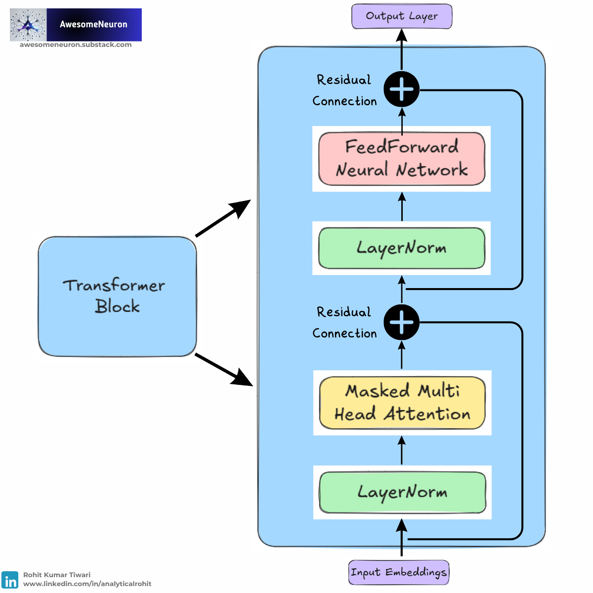
The flow through a Transformer block is:
Layer Normalization
Normalizes the input representations to improve training stability.Masked Multi-Head Attention
Allows each token to gather information from itself and previous tokens while preventing access to future tokens.Residual Connection (Add)
The original input is added back to the attention output, helping preserve information and improve gradient flow.Layer Normalization
Re-normalizes the updated representations before further processing.Feedforward Network (FFN)
Applies non linear transformations to learn more complex patterns and relationships.Residual Connection (Add)
The input from before the second Layer Normalization is added to the FFN output, preserving information while incorporating the new transformations.
Note: Dropout is often applied after the attention and feedforward operations during training. This helps reduce overfitting and improves the model’s ability to generalize.
Modern GPT models stack many transformer blocks on top of each other. Each block refines the token representations.
Here is the code showing Transformer Block in action.
class TransformerBlock(nn.Module):
    def __init__(self, embed_dim, num_heads, hidden_dim):
        super().__init__()

        self.attention = MaskedMultiHeadAttention(embed_dim, num_heads)
        self.norm1 = nn.LayerNorm(embed_dim)
        self.ffn = FeedForward(embed_dim, hidden_dim)
        self.norm2 = nn.LayerNorm(embed_dim)

    def forward(self, x):

        norm_x = self.norm1(x) # Layer normalization
        attention_output = self.attention(norm_x)  #  Multi-head causal self attention
        x = x + attention_output # Residual connections
        norm_x = self.norm2(x) # Layer normalization
        ffn_output = self.ffn(norm_x) # Feedforward neural network
        x = x + ffn_output # Residual connections

        return x
Output Layer
After passing through all the Transformer blocks, the model produces a context aware representation for each token. The model produces logits for every token position, but for next token generation it uses the logits from the final position in the sequence, which is “beginning” in this example.
This representation is then passed through the output layer:
Linear Layer (Unembedding)
The final vector is projected into a vector whose size matches the model’s vocabulary. The resulting values are called logits, with one logit for every possible token the model can generate.Softmax Function
The logits are converted into a probability distribution over the entire vocabulary. Each value now represents the model’s estimated probability of a particular token being the next token in the sequence.
The model can then select the next token. For example, if the token "." has the highest probability, it may be chosen as the prediction.
Because large language models generate text one token at a time, the predicted token is appended to the original input.
The sequence:
Every moment is a beginningbecomes:
Every moment is a beginning .This updated sequence is fed back into the model, which repeats the same process, tokenization, token embeddings, positional embeddings, transformer blocks, and output layer, to predict the next token. By repeating this cycle, the model generates text incrementally, one token at a time.
Star and Clone the GitHub Repository!
Build a ChatGPT like LLM from scratch in PyTorch, explained step by step.
Code → https://github.com/analyticalrohit/llms-from-scratch
Missed a recent post? Catch up here 👇
Liked this article? Make sure to 💜 click the like button.
Know someone that would find this helpful? Make sure to 🔁 share this post.
Get in touch
You can find me on LinkedIn | GitHub | YouTube | X | Topmate
